
Implementing Longstaff-Schwartz Least-Squares Monte Carlo for American Option Pricing
American options—contracts that can be exercised at any point before expiration—present a fundamentally harder valuation problem than their European counterparts. The early-exercise premium cannot be captured by closed-form solutions like Black-Scholes, and tree-based methods scale poorly in high dimensions. The Longstaff-Schwartz Least-Squares Monte Carlo (LSM) algorithm, introduced in 2001, elegantly bridges Monte Carlo simulation with dynamic programming to price American options and other early-exercise derivatives efficiently.
This article walks through the mechanics of LSM, its Python implementation, practical calibration considerations, and extensions relevant to quantitative finance practitioners.
Why Standard Monte Carlo Falls Short for American Options
Standard Monte Carlo simulation propagates asset paths forward in time and discounts terminal payoffs. This works perfectly for path-dependent European payoffs. However, American options require knowing the continuation value at each time step—the expected present value of holding the option rather than exercising immediately. Computing this requires backward induction, which is incompatible with forward simulation.
LSM resolves this by using ordinary least-squares regression to estimate the conditional expectation of the continuation value at each exercise date, working backward through the simulated paths.
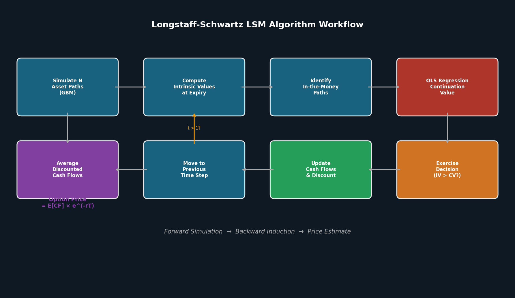
The LSM Algorithm: Step-by-Step
1. Simulate Asset Paths
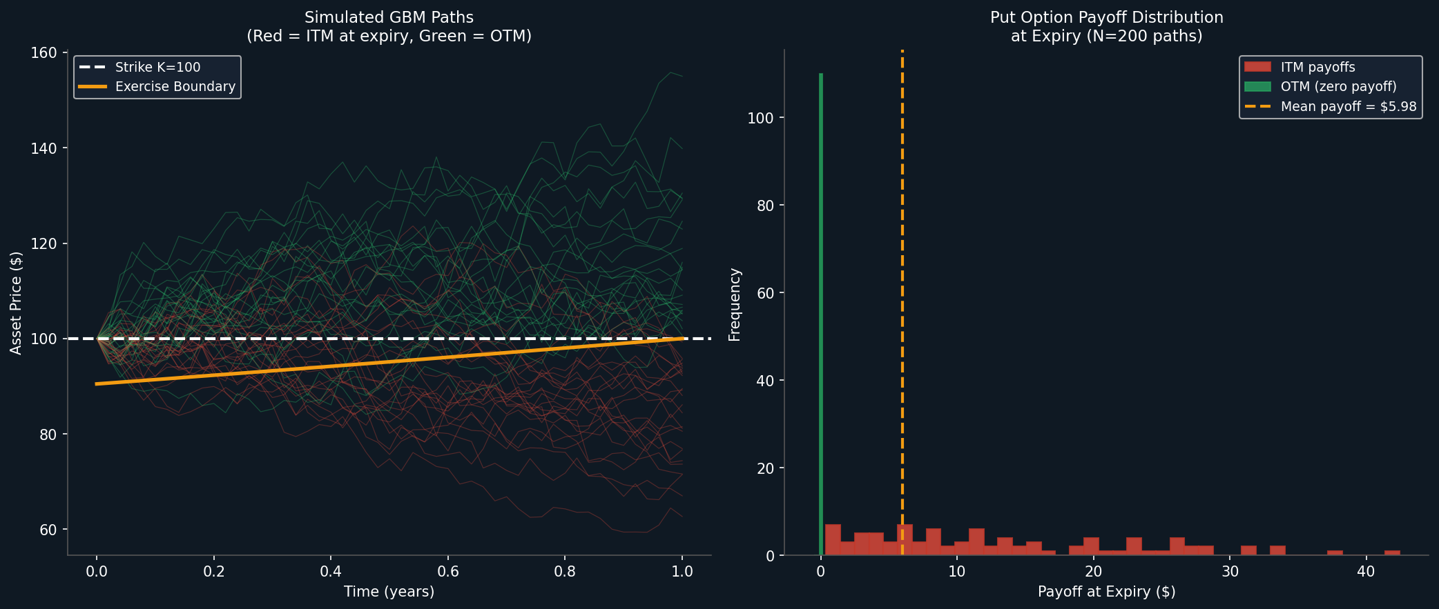
Generate N Monte Carlo paths of the underlying asset S over M time steps using Geometric Brownian Motion (or a more sophisticated model):
import numpy as np

def simulate_gbm(S0, r, sigma, T, M, N, seed=42):
    np.random.seed(seed)
    dt = T / M
    Z = np.random.standard_normal((M, N))
    S = np.zeros((M + 1, N))
    S[0] = S0
    for t in range(1, M + 1):
        S[t] = S[t-1] * np.exp((r - 0.5 * sigma**2) * dt + sigma * np.sqrt(dt) * Z[t-1])
    return S
2. Compute Intrinsic Values
For a put option with strike K, the intrinsic (immediate exercise) value at each node is:
def intrinsic_value(S, K, option_type='put'):
    if option_type == 'put':
        return np.maximum(K - S, 0)
    return np.maximum(S - K, 0)
3. Backward Induction with Regression
Starting from the final time step, work backward. At each step:
- Identify paths that are in-the-money (exercise is rational to consider).
- Regress the discounted future cash flows against basis functions of the current asset price to estimate continuation values.
- Exercise where the intrinsic value exceeds the estimated continuation value.
def lsm_american_option(S0, K, r, sigma, T, M, N, option_type='put'):
    S = simulate_gbm(S0, r, sigma, T, M, N)
    dt = T / M
    discount = np.exp(-r * dt)

    # Initialize cash flows at expiry
    CF = intrinsic_value(S[-1], K, option_type)

    # Backward induction
    for t in range(M - 1, 0, -1):
        IV = intrinsic_value(S[t], K, option_type)
        itm = IV > 0  # In-the-money paths

        if itm.sum() > 0:
            X = S[t, itm]
            Y = CF[itm] * discount  # Discounted future cash flows

            # Laguerre polynomial basis functions
            basis = np.column_stack([
                np.ones_like(X),
                X,
                X**2,
                X**3
            ])

            # OLS regression
            coeffs, _, _, _ = np.linalg.lstsq(basis, Y, rcond=None)
            continuation = basis @ coeffs

            # Exercise decision
            exercise = IV[itm] > continuation
            CF[itm] = np.where(exercise, IV[itm], CF[itm] * discount)
            CF[~itm] *= discount
        else:
            CF *= discount

    price = np.mean(CF) * discount
    return price
4. Price Estimation
The option price is the average discounted cash flow across all paths:
price = lsm_american_option(S0=100, K=100, r=0.05, sigma=0.20, T=1.0, M=50, N=100_000)
print(f"American Put Price (LSM): {price:.4f}")
For comparison, a European put under the same parameters prices at approximately $5.57 (Black-Scholes), while the American put carries an early-exercise premium, typically yielding $6.08–$6.15 depending on simulation parameters.
Basis Function Selection
The choice of regression basis functions significantly affects accuracy. Common options include:
| Basis Set | Functions | Notes |
|---|---|---|
| Laguerre polynomials | $1, x, x^2, x^3$ | Default in Longstaff-Schwartz paper |
| Hermite polynomials | $1, x, x^2-1, x^3-3x$ | Better orthogonality properties |
| Chebyshev polynomials | $T_0, T_1, T_2, T_3$ | Numerically stable for large ranges |
| Monomial + log | $1, S, S^2, \ln(S)$ | Practical for log-normal assets |
In practice, 3–5 basis functions are sufficient for single-asset options. For multi-asset or path-dependent cases, include cross-terms or use kernel regression.
Multi-Dimensional Extensions
LSM scales naturally to basket options and swing contracts by including multiple state variables in the regression:
# For a two-asset basket option
basis = np.column_stack([
    np.ones(N_itm),
    S1[itm], S2[itm],
    S1[itm]**2, S2[itm]**2,
    S1[itm] * S2[itm]  # Cross term
])
This is a key advantage over binomial/trinomial trees, which suffer from the curse of dimensionality and become computationally intractable beyond two or three assets.

Practical Calibration Tips
Convergence: Use at least 50,000–100,000 paths for stable price estimates. Variance reduction techniques (antithetic variates, control variates) can halve the required path count.
Time steps: For equity options, 50 steps per year is generally sufficient. For Bermudan options with discrete exercise dates, align steps exactly with exercise dates.
Bias: LSM produces a downward-biased price estimate because the regression approximates (rather than exactly computes) the continuation value. Combine with an upper-bound estimator (e.g., Andersen-Broadie dual method) to bracket the true price.
Antithetic variates are straightforward to implement and reduce variance by ~40% at no additional model complexity:
Z = np.random.standard_normal((M, N // 2))
Z = np.concatenate([Z, -Z], axis=1)  # Antithetic pairs
Applications Beyond Vanilla Options
LSM is the industry-standard method for pricing:
- Bermudan swaptions — callable interest rate swaps with discrete exercise dates
- Mortgage-backed securities — prepayment optionality modeled as an American option
- Real options — capital investment decisions with abandonment or expansion rights
- Commodity swing contracts — natural gas/power contracts with volume flexibility
- Variable annuities — guaranteed minimum withdrawal benefits (GMWBs)
Libraries and Tools
Several production-grade libraries implement LSM:
- QuantLib — C++/Python library with
MCAmericanEngineusing LSM - PyQL — Python bindings for QuantLib
- Riskfolio-Lib — Portfolio optimization with simulation support
- finmc — Lightweight Python Monte Carlo framework
For GPU-accelerated LSM on large path counts, CUDA-based implementations in libraries like CuPy can achieve 10–50× speedups over CPU NumPy code.
Conclusion
The Longstaff-Schwartz LSM algorithm remains the most practical and widely deployed method for pricing American and Bermudan options in production systems. Its combination of Monte Carlo flexibility with regression-based dynamic programming makes it uniquely suited for high-dimensional, path-dependent payoffs that defeat tree-based methods. Practitioners should pay careful attention to basis function selection, path count, and bias correction to achieve reliable pricing in live trading and risk management environments.
For further reading, consult the original paper: Longstaff, F.A. & Schwartz, E.S. (2001). "Valuing American Options by Simulation: A Simple Least-Squares Approach." The Review of Financial Studies, 14(1), 113–147. Available via SSRN.