
ROMS: Sediment Transport and Biogeochemical Coupling in Regional Ocean Modeling
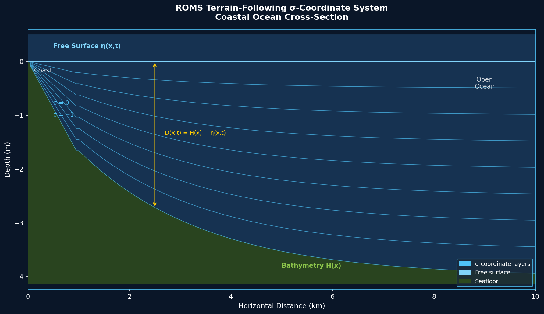
Figure 1: ROMS terrain-following σ-coordinate system. Layers conform to the bathymetry, concentrating resolution near the seafloor and free surface — critical for resolving the bottom boundary layer where sediment resuspension occurs.
The Regional Ocean Modeling System (ROMS) is a free-surface, terrain-following, primitive-equation ocean model widely adopted for coastal and regional ocean simulation. While ROMS is well known for its hydrodynamic core, its tightly integrated sediment transport and biogeochemical (BGC) modules represent some of its most powerful — and often underutilized — capabilities. This article examines how practitioners can leverage these coupled modules to simulate realistic coastal dynamics, from turbidity plumes to hypoxic zone formation.
Why Couple Sediment Transport with Hydrodynamics?
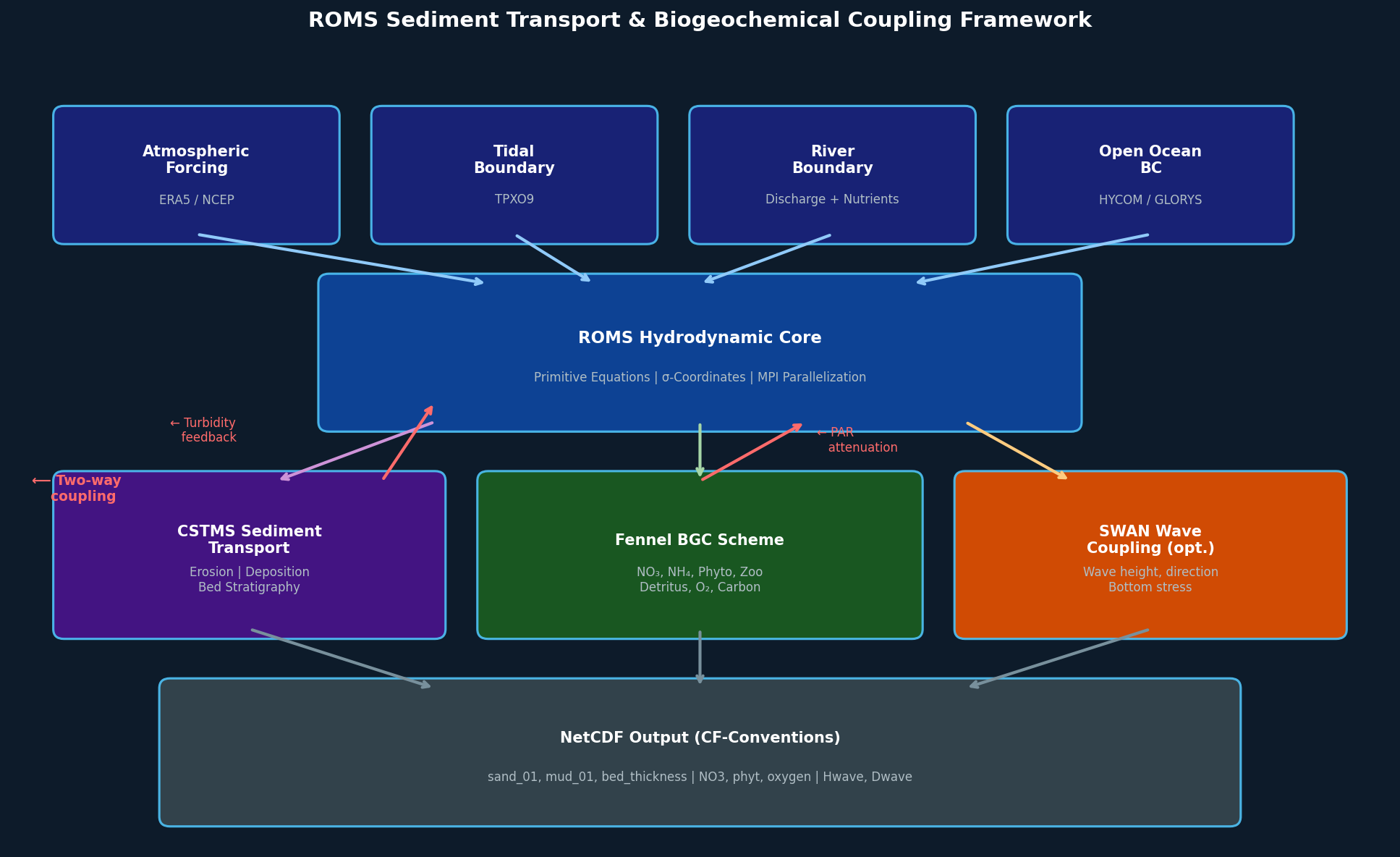
Figure 2: ROMS coupled modeling framework. The two-way feedback between the CSTMS sediment module and the Fennel BGC scheme — mediated through turbidity-driven light attenuation — is the key differentiator from loosely coupled approaches.
Coastal and estuarine environments are shaped by the interplay between water circulation, suspended particulate matter, and nutrient cycling. Treating these processes in isolation introduces significant errors: sediment resuspension alters water-column turbidity and light availability, which in turn affects primary production and oxygen demand. ROMS addresses this by coupling its hydrodynamic kernel with the Community Sediment Transport Modeling System (CSTMS) and the Fennel or BioEBUS biogeochemical schemes within a single time-stepping loop.
The key advantage is two-way feedback: sediment concentrations modify water density and light attenuation, which feeds back into the momentum equations and the BGC photosynthesis rates — all within the same model time step. This avoids the phase-lag errors that arise when running separate models and exchanging fields at coarse coupling intervals.
Setting Up the Sediment Module (CSTMS)
ROMS-CSTMS supports multiple sediment classes (cohesive and non-cohesive) defined in the sediment.in input file. Key parameters include:
Sd50— median grain diameter (m) for each sediment classSrho— sediment density (kg m⁻³)Wsed— settling velocity (m s⁻¹), which can be computed dynamically via the Stokes or van Rijn formulationsErate— erosion rate constant (kg m⁻² s⁻¹)tau_ce— critical shear stress for erosion (N m⁻²)
A typical configuration for a fine-sediment dominated estuary uses two classes: a cohesive mud fraction (Sd50 ≈ 20 µm) and a fine sand fraction (Sd50 ≈ 150 µm). The bed-layer model tracks stratigraphy through multiple active layers, enabling simulation of armoring and lag effects during storm events.
! Example sediment.in snippet (two classes)
Nbed = 3                  ! number of bed layers
Sd50 = 20.0e-6  150.0e-6  ! median grain diameter (m)
Srho = 2650.0   2650.0    ! sediment density (kg/m3)
Wsed = 0.5e-3   2.0e-3    ! settling velocity (m/s)
Erate = 5.0e-5  1.0e-4    ! erosion rate (kg/m2/s)
tau_ce = 0.05   0.10      ! critical shear stress (N/m2)
Activating Biogeochemical Coupling
ROMS supports several BGC schemes selectable at compile time via CPP flags. The Fennel et al. (2006) nitrogen-based scheme is the most commonly used for coastal eutrophication studies. It tracks nitrate, ammonium, phytoplankton, zooplankton, small and large detritus, and dissolved oxygen.
To enable sediment–BGC coupling, activate the SEDIMENT and BIOLOGY_FENNEL CPP flags together with SED_FLOCS (if flocculation is needed) in your build.sh script:
setenv MY_CPP_FLAGS "${MY_CPP_FLAGS} -DSEDIMENT"
setenv MY_CPP_FLAGS "${MY_CPP_FLAGS} -DBIOLOGY_FENNEL"
setenv MY_CPP_FLAGS "${MY_CPP_FLAGS} -DOXY"
setenv MY_CPP_FLAGS "${MY_CPP_FLAGS} -DCARBON"
The coupling pathway works as follows: suspended sediment concentrations computed by CSTMS are passed to the light attenuation subroutine, where they contribute to the total diffuse attenuation coefficient Kd alongside chlorophyll and CDOM. This directly modulates the photosynthetically available radiation (PAR) reaching each depth layer, suppressing phytoplankton growth in turbid conditions — a critical process in river plume and estuarine front dynamics.
Practical Workflow: Simulating a Hypoxic Event
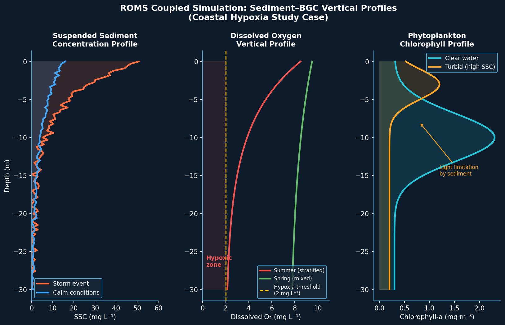
Figure 3: Representative ROMS coupled simulation output. Left: suspended sediment concentration (SSC) profiles under storm vs. calm conditions. Center: dissolved oxygen profiles showing summer hypoxia below the 2 mg L⁻¹ threshold. Right: chlorophyll-a profiles illustrating light limitation of phytoplankton growth in turbid water.
A representative use case is simulating seasonal bottom-water hypoxia in a stratified coastal embayment. The recommended workflow is:
- Spin-up the hydrodynamic model for 1–2 years using climatological forcing (NCEP or ERA5 atmospheric fields, tidal constituents from TPXO) to establish a stable density field.
- Add river boundary conditions with observed discharge, suspended sediment load, and nutrient concentrations from USGS gauge data.
- Enable the BGC module and run through the spring bloom period, monitoring surface chlorophyll against satellite-derived estimates (MODIS Aqua, Sentinel-3 OLCI) for validation.
- Activate sediment resuspension and examine the feedback on light limitation and benthic oxygen demand (BOD) parameterized through the
bfluxbottom boundary condition. - Diagnose hypoxia by tracking dissolved oxygen fields against the 2 mg L⁻¹ threshold and comparing spatial extent with observational surveys.
Grid resolution is a critical consideration: resolving the halocline and pycnocline that trap low-oxygen water typically requires vertical layers concentrated near the bottom (terrain-following σ-coordinates with Vstretching = 4, Vtransform = 2, and theta_b ≈ 3.0).
Performance and Parallelization
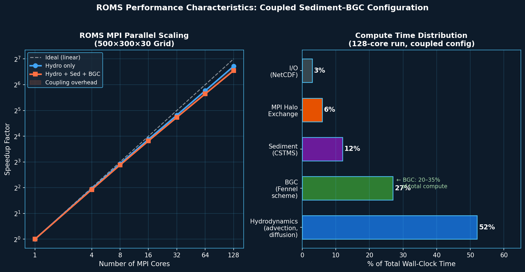
Figure 4: ROMS performance characteristics for a 500×300×30 grid with coupled sediment and BGC. Left: MPI scaling efficiency showing near-linear speedup to 128 cores. Right: compute time breakdown — BGC accounts for ~27% and sediment transport ~12% of total wall-clock time.
ROMS is parallelized via MPI domain decomposition. For a 500 × 300 × 30 grid with two sediment classes and the Fennel BGC scheme, expect roughly 3–5× longer wall-clock time compared to the hydrodynamic-only configuration. Profiling with the built-in PROFILE CPP flag reveals that the BGC routines typically account for 20–35% of total compute time, while sediment advection–diffusion adds another 10–15%.
Optimal tile decomposition follows the rule of thumb: NtileI × NtileJ ≈ number of MPI tasks, with each tile containing at least 20 grid points per dimension to amortize halo-exchange overhead. On a 128-core cluster, a 16 × 8 decomposition typically yields near-linear scaling efficiency above 85%.
Validation and Output
ROMS writes NetCDF output compatible with CF conventions, making post-processing straightforward with Python (xarray, matplotlib) or MATLAB. Key diagnostic variables for sediment–BGC studies include:
sand_01,mud_01— depth-averaged suspended sediment concentrationsbed_thickness— total active bed layer thicknessNO3,phyt,zoop— Fennel BGC state variablesoxygen— dissolved oxygen (mmol O₂ m⁻³)Hwave,Dwave— wave height and direction (if SWAN coupling is active)
The ROMS Wiki provides comprehensive documentation on input file formats, CPP flags, and test cases. The ROMS Forum is an active community resource for troubleshooting coupled configurations.
Key Takeaways
ROMS's integrated sediment transport and biogeochemical modules provide a physically consistent framework for simulating the complex feedbacks that govern coastal water quality. By coupling CSTMS with the Fennel BGC scheme, practitioners can capture turbidity-driven light limitation, nutrient-driven eutrophication, and benthic oxygen demand within a single model framework — capabilities that are essential for regulatory applications such as TMDL (Total Maximum Daily Load) assessments and coastal hypoxia management. The investment in configuring the coupled system pays dividends in simulation fidelity that standalone hydrodynamic or BGC models simply cannot match.